Kappa Vault

This article expands on “Data Vault Agility on Snowflake”; see: bit.ly/337Jhp3, scroll down to “Multiple source system cadence and how to handle it”
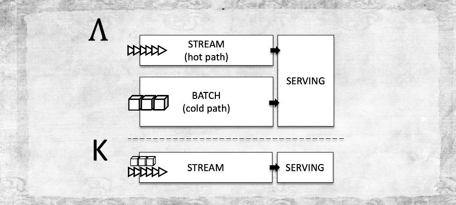
What is Kappa Architecture?
Coined by Jay Kreps back in 2014 (see: bit.ly/3CtWZQo) Kappa challenges the thinking and design behind a Lambda architecture. The premise behind Lambda is the separation of batch and streaming workloads defined as batch and speed layers respectively. If you wanted data now then you must accept a margin of error in the results, batch will “catch up” and consolidate the data in the serving layer with a higher degree of accuracy. This is an implementation of eventual consistency. Kappa on the other hand is a stream first approach, both workloads are handled by a single stream processing engine that can deal with batch and streaming, something Snowflake today natively supports with Snowpipe and Kafka, see: bit.ly/3fqV9oZ.
A vast array of algorithms has been developed through the years that incorporates this margin of error in stream-only analytics and all with the same principle in mind; if you want the answer now it might not be accurate, if you want it later sure we can provide that accuracy you desire later.
Snowflake provides a suit of estimation functions that include:
- HyperLogLog for cardinality estimation, see: bit.ly/35JKaWo
- MinHash for similarity estimation between two sets, see: bit.ly/3hZ58CW
- Space-saving algorithm for estimation of frequent values, see: bit.ly/3MM7LGg
- t-Digest for approximate percentiles, see: bit.ly/34Bt38z
Use of these functions and techniques becomes necessary when the volume of data becomes unfeasible to run the otherwise exact functions.
Is Data Modelling Dead?
Famously quipped on dbt discourse is the notion of defining Data Vault and Kimball modelling as “irrelevant” data modelling methodologies, instead rely on flat wide marts using the data platform’s columnar optimizations to negate the need to use those legacy techniques. It is amusing that we see some data modelling techniques appear as ground-breaking today that were in fact solved for years ago, but with a smaller volume of data. And that is true of Data Vault too, sure in a Big Data platform building a Data Vault that is essentially change-based proves to be a challenging and complex task but with the release of Snowflake those challenges melt away. Snowflake’s unique patented technology breaks down what used to be very large immutable files into tens to thousands of 16MB immutable files that make up a table, and all of it managed and tracked via FoundationDB as metadata. This breathes new life into the “old” data modelling techniques by suddenly providing these methodologies with the unlimited scalability of the Data Cloud and the flexibility of an OLAP SQL engine. And for Data Vault these are documented here:
- The use of hash-keys for data distribution on a Massively Parallel Platform (see: bit.ly/3dn83n8), we highlight why hash keys are still a relevant construct in Snowflake
- Point-in-time (PIT) tables that uses Kimball modelling efficiencies to achieve a Right-Deep Join tree for efficient OLAP querying over a Data Vault (see: bit.ly/3dBxOQK),
- Conditional multi-table inserts for PIT tables that provides a single-source optimised pipeline for creating snapshots of the Data Vault hubs, links, and satellites (see: bit.ly/3iEkBJC),
- Accelerating Data Vault loading pipelines with inherent hub table transaction locking and dynamic pruning for getting the data out (see: bit.ly/337Jhp3)
- Efficiently automated testing your Data Vault using Snowflake cloud services’ metadata and streams on tables. (see: bit.ly/3dUHPIS),
- Time-line correction for data being presented out of sequence (see: bit.ly/3aCCRhQ), and
- Snowsight dashboards on a Data Vault test framework (see: bit.ly/3BjSg1F)

In reality there is always a data model, relational or non-relational the data model represents how we represent the data to model the business process. Whether it is relational or non-relational depends largely on what can be achieved with the highest degree of efficiency. Semi-structured data avoids the need to model column names and data types up-front where such an effort would delay business value to an inefficient extent. Make no mistake though, having those columns and data types defined in a structured table will be more efficient to understand and query from the business point of view, but is it necessary to model all these elements if they are not considered critical data elements (CDEs)? Semi-structure data does have a data model, the agreed upon key-value pairs, but it does not enforce data typing. Snowflake of course can natively read semi-structured data using its SQL syntax without the need to pre-parse them! (see: bit.ly/3KUTZQf).
For a concise understanding of where Data Vault fits follow the breadcrumbs to these articles:
- Combining Business Architecture and Data Vault, see: bit.ly/3fUL7fN
- Bread and Data Vault, see: bit.ly/2WEWCSw
Streams on Views
Building data models based on ever-growing full table scans is an obvious anti-pattern if the growth runs into the terabytes or more! To circumvent this pattern data engineering teams must implement orchestration of landed files (push or pull, log-scraping) and purging and or archiving of data already consumed by the target data platform. The rule for loading a data model based on change detection is that you can only process one file at a time, why? That single file has an applied/extract date and the data loaded in the correct order is compared to what is the current record per parent-key in the target satellite table, only new change-records are loaded. Snowflake Streams on the other hand, gives us a way to minimalize the data being processed downstream of landed data. Snowflake’s streams capability drives your Snowflake architecture ever so closer to realising your Kappa architecture entirely within Snowflake itself. Introduced circa 2020 Snowflake streams can be thought of as the equivalent of Change Data Capture (CDC) on Microsoft SQL Server by adding additional tracking columns to denote the actions that were performed to a record on the underlying table; and that is where the similarity ends.
What is the same is that there are additional metadata only columns visible to the user of the stream, in Snowflake these are,
- METADATA$ACTION — INSERT or DELETE
- METADATA$ISUPDATE — TRUE or FALSE if the action above was the result of an update or not
- METADATA$ROW_ID –a GUID uniquely identifying the row
Like traditional CDC we can either track append-only changes or insert, updates and deletes.
What is different is that the addition of a stream adds a place marker to the underlying table; if you create an empty table and add the place marker then any new data added to the table is visible to the user of the place marker. If you create a table and add the place marker after you have loaded data to it then to the user of this other place marker the table appears empty, because the place marker is added on the table as it appears in that state, at the end. However, when data is added to the table that new data will be visible by both place markers.

Creating a placeholder on the table object
create stream <stream-name> on table <table-name>;
Creating a placeholder using Time Travel
create stream <stream-name> on table <table-name> at (timestamp => to_timestamp_tz(‘01/01/2022 09:02:03’, ‘mm/dd/yyyy hh24:mi:ss’));
Standard Time Travel statements apply
Running a SELECT statement on the place marker does not “consume” it, in other words it does not advance the place marker to the end of the stream. Only if the place marker is consumed by way of using a Data Manipulation Language (DML) statement does the place holder get consumed (advanced to the end of the table), a DML statement reads data from the stream and loads that output to another table (with transformations if applicable) — the data streams from one table to another. Let’s demonstrate by way of illustration.

This now reduces the amount of data into a stream of data for downstream processing. You are also not restricted to where you can add your place marker, you can define where to insert that place marker based on time travel (previous state of the table) by simply adding a time stamp denoting the state of that data at that date. What’s more is that Snowflake’s streams are not limited to Snowflake tables, at the time of writing you can create a Snowflake stream on:
- Data Share, a unique concept other vendors want to replicate, the ability to instantly share data from one Snowflake account to another. Data from one Snowflake account appears in realtime to another account the data is shared with.
- External Table, yes, Snowflake can track what are new records to a supported External Table. CSV, JSON, AVRO, Parquet and ORC.
- Directory Tables, specific to Snowflake’s support for unstructured data, the directory table is created to track these blob files loaded into Snowflake’s Internal Stage, see: bit.ly/3pY2bHi, yes, being able to track new unstructured data loaded to Snowflake stages!
- Views, the subject matter of this section and why it is such a powerful feature added to Snowflake’s repertoire!
Streams on Views introduces an opportunity to build a true real time Data Vault loading pattern.

The traditional approach to loading a data vault relies on a single landed file and loading it before the next file is landed. The landed content is staged with data vault tags such as load dates, record source, record-hash, and surrogate hash keys. Every file landed will also have an applied date, the date that this package of business process outcomes is applicable to. If staging is deployed as a view, then no additional data movement is needed for staging. That staged content is then loaded to target hubs, links and satellites and condensed using “select distinct” for each target to ensure target table integrity.
The problem occurs when data is being loaded faster than the hub, link and satellite loaders can ingest them, three predominant approaches to loading these have survived
- Looping multiple files through the entire staging to load orchestration if each new package of data is loaded as a separate file. The downside is that the entire orchestration must wait for all the downstream loaders to complete for each file before processing the next file.

2. Looping within a single file; if separate files are not used but instead simply appended to a single file; for each applied date in the file the data is looped against the target tables by the oldest record first, thereby ensuring true changes are loaded to the target tables. The downside of this approach is the new data cannot be landed while this looping occurs (unless you use a control table — more complexity), and the approach requires what could be expensive data chunking to check against the target table multiple hits for a single load. Of course, this approach can use a stream on the table to only process new data, more on this later.

3. Defining a business date as an intra-day key; this avoids looping but may load non-true changes to the target satellite tables. The load code modification is very simple, designate a business date in the source as the dependent-child-key for a satellite table then let the loader use that in the comparison operator itself. However, not all landed data will have a reliable business date to define as an intra-day key and the approach does suffer from the same shortcoming as above, it relies on nothing being loaded to the landed file until the loader has completed. The other possible shortcoming is in the case of satellite splitting, is there a consistent approach to including intra-day keys to both split satellites or does one satellite not need that intra-day key and the other does? Does the loading pattern now impose a data model change? Loading patterns should never dictate what the data model should be!

Streams on Views does something different for us; because it is based on the view itself the data already applies the necessary data vault tags when being ingested downstream. For each target table a placeholder is created, if the source is meant to load a hub and satellite table then a stream will exist on the view for each. For each loader a common table expression (CTE) is used right before the loader is used to condense the incoming records. This condensing removes duplicates by parent key and the loader itself will compare the oldest record by parent key in the CTE output to keep or discard that record before the loader source-to-target comparison. All other records for a parent key are loaded because they have already been condensed in the CTE.

Why use this approach?

Why not deploy a stream on the table instead and deploy multiple views to add the data vault tags? Well, for each target data vault table you have replicated hash creation and therefore multiplied the cost to create those surrogate hash keys. Remember, a hub hash key will be loaded to a target hub table and a target satellite table, why calculate this twice?
Why not deploy a single view over a stream that’s based on a table? The issue here comes down to ownership, if the owner of the view is different to the owner of the stream, then how do we manage the placeholders and advancing that placeholder? Sure, if the owner is the same then this might be feasible pattern for you. It is however an anti-pattern
A Stream on the View with CTEs to apply the condensing of the data before loading allows you to:
- Isolate the calculation of hashes (record hash and surrogate hash keys) to a single place, rather than replicate the same logic in multiple places!
- Satellite splitting means you cannot apply record condensing in that single stage, but rather have those configured by their respective targets, hence having multiple streams on views and each autonomous CTE deal with the duty of discarding duplicates per satellite split.
— hub condensed CTE discards duplicate surrogate-hub-hash keys to ensure we load a distinct list of new keys, with the oldest applied date
— link condensed CTE discards duplicate surrogate-link-hash keys to ensure we load a distinct list of new keys, with the oldest applied date
— satellite condensed CTE will have discard duplicate record attributes based on a satellite split, this checks the current record-hash against the previous record-hash by parent key (hub or link). If the previous record-hash and current record-hash are the same, then discard the record
- Relies on Snowflake native technology to manage placeholders and advancement of placeholders and there is no need to wait for loading to target hubs, links, and satellites to complete before loading more data into the landed file. If more data is landed while we load, the next stream ingestion simply pulls from that placeholder and advances the placeholder to the end of the view — we have essentially removed the dependency between landing and loading and simplified the overall orchestration.
- The overall orchestration is reduced to simply deploying code to snowflake and is then triggered by a single “insert into” statement for each target table, and you do not need to code anything outside of this statement to automate this orchestration. The loaders are executed in parallel and reconciliation checks are executed as the content completes their loads.
How to apply this approach

Break down the elements needed to function autonomously, scalable, and idempotent and you have automation. The number of elements needed to deliver a single hub table with no descriptive content is achieved by setting these minimum number of elements in Snowflake, mind you, you still need to configure things like business key collision codes (if needed), mapping source business keys to target business key hub column, tenant id… oh my! See: bit.ly/3bRlV7U
What are the minimum elements needed in this approach for a hub?

- View to add the data vault tags described above (stage view is 1:1 with the table object),
stg_${src-badge}_${src-file}
for example stg_card_masterfile
- A Snowflake Stream on the View (stream on view is 1:1 with the target table)
str_${src-badge}_${src-file}_to_hub_${hub-name}_ ${hub-key-name}
for example, str_card_masterfile_to_hub_account_dv_hashkey_hub_account
- A Snowflake task to execute the loader (task will be 1:1 with the stream)
tsk_${src-badge}_${src-file}_to_hub_${hub-name}_ ${hub-key-name}
for example, tsk_card_masterfile_to_hub_account_dv_hashkey_hub_account
That’s right, set and forget, Snowflake tasks feature (see: bit.ly/3J6u2wz) was released at the same time Snowflake Streams were that act like cattle herders for your streams. They execute standard Snowflake SQL and can be daisy chained into multiple SQL statements or use the Snowflake task to execute a Snowflake Stored Procedure. What it means in this context is simply deploying these elements above and the orchestration is executed when the task runs the respective loader code (also parameterized). The loader will consume the stream on the view that includes all the relevant configured data vault tags and discard duplicates along the way! The cadence of the task to execute these independent loaders is set by you.


- For status tracking and effectivity satellites secondary staging is no longer needed, inferring deletes is now pushed to the CTE.
- For non-historized links and satellites the loaders do not need to check if the incoming record is new, by definition it always is. It also means that likely you do not need the CTEs to discard duplicates (condensing) but the stream on view is still immensely useful!
- For the automated test framework, these must be amended to check between landed content and target table by applied date, data should always be loaded in applied date order and therefore it is likely you achieve efficient pruning on Snowflake tables.
- At the time of writing, Snowflake tasks does have a limitation allowing a single task from having multiple parents that prevent it from being a true Direct Acyclical Graph (DAG). This is needed for executing orphan checks.
The Omega
Data Vault 2.0 is INSERT only, this is the most efficient data modelling pattern even for change records; the point in time querying of data vault is handled and managed at query time. Previous articles highlighted how to query a data vault efficiently and build Information Mart views over your Raw and Business Vault. This also means your streams should be implemented as APPEND or INSERT ONLY, there really is no need to track updates and deletes because in Data Vault we do not delete data. For your landed content do we delete old data? Well aside from regulatory requirements, you don’t need to (check with your business users what those requirements are).
Snowflake’s approach to breaking down tables into encrypted and compressed immutable files achieves columnar and row-level compression whose storage footprint cost is similar to a blob file stored in AWS Glacier. That’s right, yet another amazing feature of Snowflake technology that if you can avoid registering external tables at all you can take full advantage of Snowflake’s features.
Snowflake’s features are intended to be easy-to-use, and in my opinion, they are. You are not managing clusters, vacuuming tables to recover storage, or ensuring your table indexes are performing efficiently. You are also not constrained to the number of concurrent users who can query the data while it is being loaded. Even table locking is inherently achieved when multiple pipelines are loading shared hub tables, see: bit.ly/337Jhp3. The cost of storing your data is passed onto you, and Snowflake uses a pay-as-you-go model for computations ensuring that if you understand the fundamental building objects Snowflake affords you to design and deploy to your desires, you can easily establish an agile set of repeatable patterns to deliver your analytics in real time.
Reference
- Big data architectures, see: bit.ly/3HXHXDu
- Get your Symbols, see: https://wumbo.net/
#thedatamustflow #datavault #snowflake #snowsight #kappavault
The views expressed in this article are that of my own, you should test implementation performance before committing to this implementation. The author provides no guarantees in this regard.